Decoding Multidimensional Gradient

Gradec provides .

# Download HCP S1200 principal gradient
from gradec.fetcher import _fetch_gradients

gradients = _fetch_gradients(cortical=True)

Multidimensional Segmentation

Select the first four gradients

gradients_4d = gradients[:, :4]

KMeans-based segmentation

from surfplot.utils import add_fslr_medial_wall

from gradec.plot import plot_surf_maps
from gradec.segmentation import KMeansSegmentation

full_vertices = 64984
hemi_vertices = full_vertices // 2

segmentation = KMeansSegmentation(n_segments=4)
segmentation.fit(gradients_4d)
grad_maps = segmentation.transform()

Multidimensional Decoding

from gradec.decode import LDADecoder
from gradec.fetcher import _fetch_classification, _fetch_features, _fetch_frequencies
from gradec.plot import plot_cloud
from gradec.utils import _decoding_filter

SPACE, DENSITY = "fsLR", "32k"
DSET, MODEL = "neuroquery", "lda"

# Fit the decoder
decode = LDADecoder(space=SPACE, density=DENSITY, calc_pvals=False)
decode.fit(DSET)

# Load features for visualization
features = _fetch_features(DSET, MODEL)
frequencies = _fetch_frequencies(DSET, MODEL)
classification, class_lst = _fetch_classification(DSET, MODEL)

Decode map

corrs_df = decode.transform(grad_maps, method="correlation")

0%|          | 0/4 [00:00<?, ?it/s]
0%|          | 0/4 [00:00<?, ?it/s]

Visualize results

cmaps = ["Blues", "Greens", "Greys", "Reds"]
for map_i, (grad_map, segment) in enumerate(zip(grad_maps, corrs_df.columns)):
    seg_df = corrs_df[[segment]]
    # Filter results
    filtered_df, filtered_features, filtered_frequencies = _decoding_filter(
        seg_df,
        features,
        classification,
        freq_by_topic=frequencies,
        class_by_topic=class_lst,
    )
    filtered_df.columns = ["r"]
    corrs = filtered_df["r"].to_numpy()

    # Gradient map plot
    grad_map = add_fslr_medial_wall(grad_map)
    grad_map_lh, grad_map_rh = (
        grad_map[:hemi_vertices],
        grad_map[hemi_vertices:full_vertices],
    )
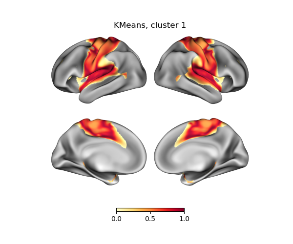
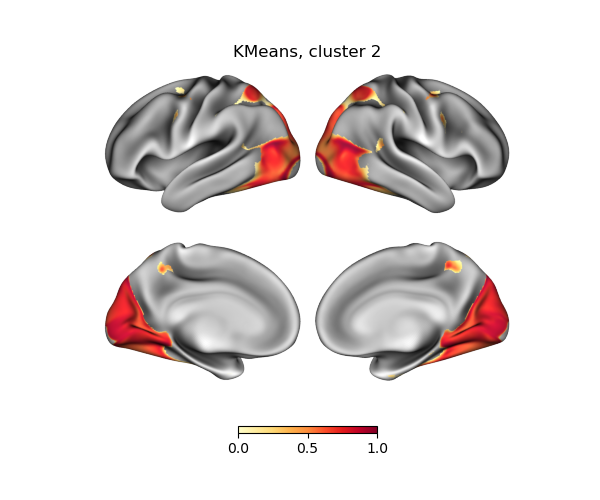
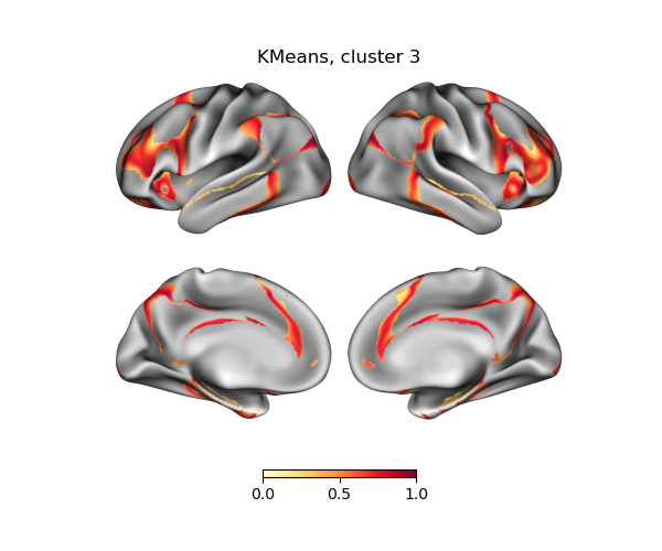
    fig = plot_surf_maps(
        grad_map_lh,
        grad_map_rh,
        color_range=(0, 1),
        cmap="YlOrRd",
        title=f"KMeans, cluster {map_i+1}",
    )
    fig.show()

    # Word cloud plot
    cloud_fig = plot_cloud(
        corrs,
        filtered_features,
        MODEL,
        frequencies=filtered_frequencies,
        cmap=cmaps[map_i],
    )
    cloud_fig.show()

• 
• 
• 
• 
• 
• 
• 
•